Importing receptor data into scirpy#
Show code cell content
# This cell is for development only. Don't copy this to your notebook.
%load_ext autoreload
%autoreload 2
import anndata

anndata.logging.anndata_logger.addFilter(
    lambda r: not r.getMessage().startswith("storing") and r.getMessage().endswith("as categorical.")
)

# Temporarily suppress FutureWarnings
import warnings

warnings.simplefilter(action="ignore", category=FutureWarning)
import tarfile
import warnings
from glob import glob

import anndata
import matplotlib.pyplot as plt
import muon as mu
import pandas as pd
import scanpy as sc
import scirpy as ir

sc.set_figure_params(figsize=(4, 4))
sc.settings.verbosity = 2  # verbosity: errors (0), warnings (1), info (2), hints (3)
In this notebook, we demonstrate how single-cell AIRR-data can be imported into
an AnnData object and merged with gene expression data in a MuData container for the use with Scirpy.
To learn more about how AIRR data is represented in AnnData, check out the data structure section.
Important
The scirpy data model
Since v0.13, there are no restrictions on the AIRR data that can be stored in the scirpy data structure, except that each receptor chain needs to be associated with a cell. However, for all analyses, the assumptions of the receptor model still apply:
BCR and TCR chains are supported. Chain loci must be valid Chain locus, i.e. one of
TRA,TRG,IGK, orIGL(chains with a VJ junction) orTRB,TRD, orIGH(chains with a VDJ junction).Each cell can contain up to two
VJand twoVDJchains (Dual IR). Excess chains are ignored (those with lowest read count/UMI count) and cells flagged as Multichain-cell.Non-productive chains are ignored. CellRanger, TraCeR, and the AIRR rearrangment format flag these cells appropriately. When reading custom formats, you need to pass the flag explicitly or filter the chains beforehand.
The index_chains() function chooses the appropriate chains for each cell according to this model
and stores references to those chains in adata.obsm.
Note
AIRR quality control
After importing the data, we recommend running the
scirpy.tl.chain_qc()function. It will 1. identify the Receptor type and Receptor subtype and flag cells asambiguousthat cannot unambigously be assigned to a certain receptor (sub)type, and 2. flag cells with orphan chains (i.e. cells with only a single detected cell) and multichain-cells (i.e. cells with more than two full pairs of VJ- and VDJ-chains).We recommend excluding multichain- and ambiguous cells as these likely represent doublets
Based on the orphan chain flags, the corresponding cells can be excluded. Alternatively, these cells can be matched to clonotypes on a single chain only, by using the
receptor_arms="any"parameter when runningscirpy.tl.define_clonotypes().
Loading data from estabilshed analysis pipelines or AIRR-compliant tools#
We provide convenience functions to load data from 10x CellRanger, BD Rhapsody, TraCeR, or BraCeR with a single function call. Moreover, we support importing data in the community-standard AIRR rearrangement schema.
|
Read AIRR data from 10x Genomics cell-ranger output. |
|
Read data from TraCeR ([SLonnbergP+16]). |
|
|
|
Read data from AIRR rearrangement format. |
|
Read IR data from the BD Rhapsody Analysis Pipeline. |
|
Read 10x data#
With read_10x_vdj() we can load filtered_contig_annotations.csv or contig_annotations.json files as they are produced by CellRanger.
Here, we demonstrate how to load paired single cell transcriptomics and TCR sequencing data from COVID19 patients
from GSE145926 [LLY+20].
# Load the TCR data
adata_tcr = ir.io.read_10x_vdj("example_data/liao-2019-covid19/GSM4385993_C144_filtered_contig_annotations.csv.gz")

# Load the associated transcriptomics data
adata = sc.read_10x_h5("example_data/liao-2019-covid19/GSM4339772_C144_filtered_feature_bc_matrix.h5")
adata.var_names_make_unique()
reading example_data/liao-2019-covid19/GSM4339772_C144_filtered_feature_bc_matrix.h5
 (0:00:00)
This particular sample only has a detected TCR for a small fraction of the cells:
adata_tcr.shape
(136, 0)
adata.shape
(3716, 33539)
Next, we integrate both the TCR and the transcriptomics data into a single MuData object. By convention,
gene expression data should be stored in the gex modality, immune receptor data in the airr modality.
mdata = mu.MuData({"gex": adata, "airr": adata_tcr})
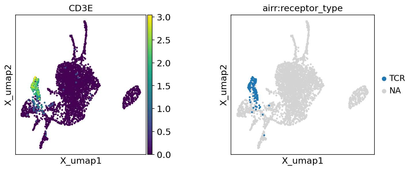
Now, we can use TCR-related variables together with the gene expression data. Here, we visualize the cells with a detected TCR on the UMAP plot. It is reassuring that the TCRs coincide with the T-cell marker gene CD3.
sc.pp.log1p(mdata["gex"])
sc.pp.pca(mdata["gex"], svd_solver="arpack")
sc.pp.neighbors(mdata["gex"])
sc.tl.umap(mdata["gex"])
computing PCA
    with n_comps=50
    finished (0:00:02)
computing neighbors
    using 'X_pca' with n_pcs = 50
    finished (0:00:01)
computing UMAP
    finished (0:00:06)
ir.pp.index_chains(mdata)
ir.tl.chain_qc(mdata)
Stored result in `mdata.obs["airr:receptor_type"]`.
Stored result in `mdata.obs["airr:receptor_subtype"]`.
Stored result in `mdata.obs["airr:chain_pairing"]`.
Read Smart-seq2 data processed with TraCeR#
TraCeR [SLonnbergP+16] is a method commonly used to extract TCR sequences from data generated with Smart-seq2 or other full-length single-cell sequencing protocols.
The scirpy.io.read_tracer() function obtains its TCR information from the .pkl file
in the filtered_TCR_seqs folder TraCeR generates for each cell.
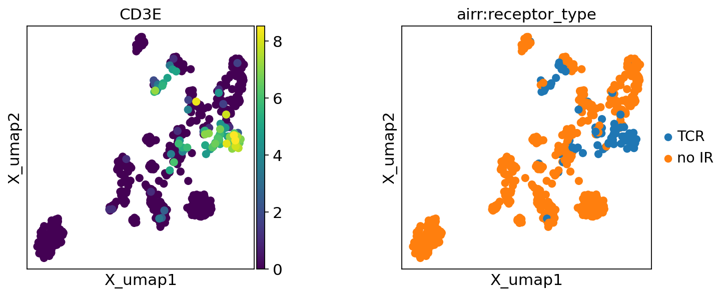
For this example, we load the ~500 cells from triple-negative breast cancer patients from GSE75688 [CEL+17]. The raw data has been processed using the Smart-seq2 pipeline from nf-core.
# extract data
with tarfile.open("example_data/chung-park-2017.tar.bz2", "r:bz2") as tar:
    tar.extractall("example_data/chung-park-2017")
First, we load the transcriptomics data from the counts.tsv file:
expr_chung = pd.read_csv("example_data/chung-park-2017/counts.tsv", sep="\t")
# anndata needs genes in columns and samples in rows
expr_chung = expr_chung.set_index("Geneid").T
adata = sc.AnnData(expr_chung)
adata.shape
(563, 23438)
Next, we load the TCR data and merge it with the transcriptomics data:
adata_tcr = ir.io.read_tracer("example_data/chung-park-2017/tracer/")
mdata = mu.MuData({"gex": adata, "airr": adata_tcr})
sc.pp.highly_variable_genes(mdata["gex"], flavor="cell_ranger", n_top_genes=3000)
sc.pp.log1p(mdata["gex"])
sc.pp.pca(mdata["gex"], svd_solver="arpack")
sc.pp.neighbors(mdata["gex"])
sc.tl.umap(mdata["gex"])
ir.pp.index_chains(mdata)
ir.tl.chain_qc(mdata)
If you pass `n_top_genes`, all cutoffs are ignored.
extracting highly variable genes
    finished (0:00:00)
computing PCA
    on highly variable genes
    with n_comps=50
    finished (0:00:00)
computing neighbors
    using 'X_pca' with n_pcs = 50
    finished (0:00:00)
computing UMAP
    finished (0:00:01)
Stored result in `mdata.obs["airr:receptor_type"]`.
Stored result in `mdata.obs["airr:receptor_subtype"]`.
Stored result in `mdata.obs["airr:chain_pairing"]`.
Read an AIRR-compliant rearrangement table#
We generated example data using immuneSIM [WAY+20]. The data consists of 100 cells and does not include transcriptomics data.
The rearrangement tables are often organized into separate tables per chain. Therefore, scirpy.io.read_airr() supports
specifiying multiple tsv files at once. This would have the same effect as concatenating them before
the import.
adata = ir.io.read_airr(
    [
        "example_data/immunesim_airr/immunesim_tra.tsv",
        "example_data/immunesim_airr/immunesim_trb.tsv",
    ]
)
ir.pp.index_chains(adata)
ir.tl.chain_qc(adata)
Stored result in `adata.obs["receptor_type"]`.
Stored result in `adata.obs["receptor_subtype"]`.
Stored result in `adata.obs["chain_pairing"]`.
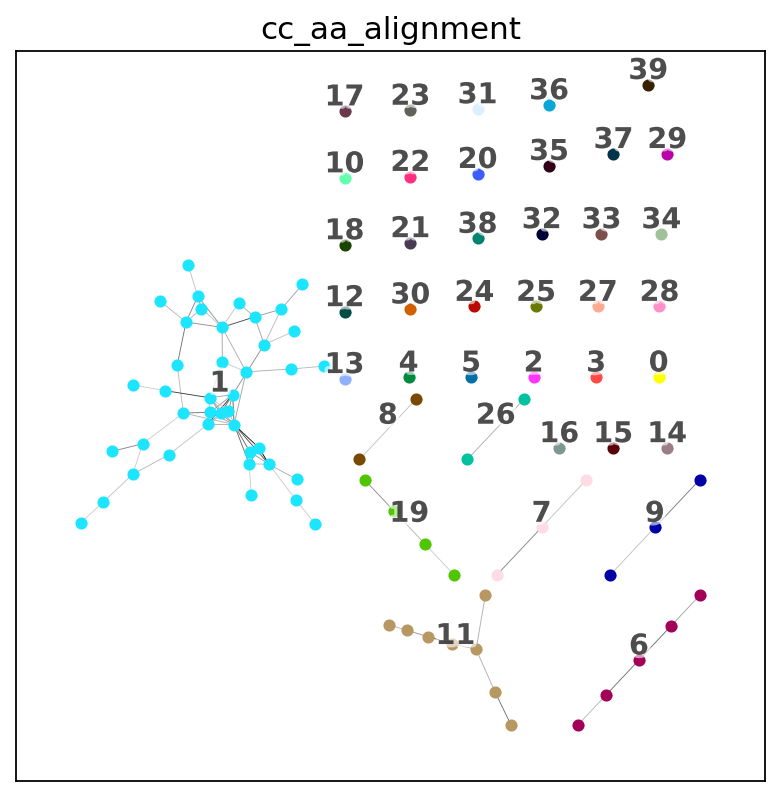
The dataset does not come with transcriptomics data. We can, therefore, not show the UMAP plot highlighting cells with TCRs, but we can still use scirpy to analyse it. Below, we visualize the clonotype network connecting cells with similar CDR3 sequences.
Note: The cutoff of 25 was chosen for demonstration purposes on this small sample dataset. Usually a smaller cutoff is more approriate.
ir.pp.ir_dist(adata, metric="alignment", sequence="aa", cutoff=25)
Computing sequence x sequence distance matrix for VJ sequences.
Computing sequence x sequence distance matrix for VDJ sequences.
ir.tl.define_clonotype_clusters(
    adata,
    metric="alignment",
    sequence="aa",
    receptor_arms="any",
    dual_ir="primary_only",
)
ir.tl.clonotype_network(adata, size_aware=False, metric="alignment", sequence="aa")
ir.pl.clonotype_network(
    adata,
    color="cc_aa_alignment",
    base_size=20,
    panel_size=(6, 6),
    show_legend=False,
    show_size_legend=False,
)
Creating AnnData objects from other formats#
Often, immune receptor (IR) data are just provided as a simple table listing the CDR3 sequences for each cell.
We provide a generic data structure for cells with IRs, which can then be converted into
an AnnData object.
|
Data structure for a Cell with immune receptors. |
|
If you believe you are working with a commonly used format, consider sending a feature request
for a read_XXX function.
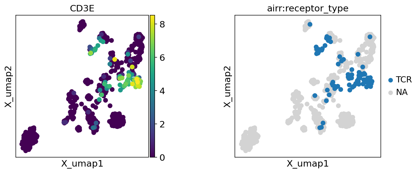
For this example, we again load the triple-negative breast cancer data from [CEL+17]. However, this time, we retrieve the TCR data from a separate summary table containing the TCR information (we generated this table for the sake of the example, but it could very well have been a supplementary file from the paper).
Such a table typically contains information about
CDR3 sequences (amino acid and/or nucleotide)
The Chain locus, e.g.
TRA,TRB, orIGH.expression of the receptor chain (e.g. count, UMI, transcripts per million (TPM))
the V(D)J genes for each chain
information if the chain is productive.
tcr_table = pd.read_csv(
    "example_data/chung-park-2017/tcr_table.tsv",
    sep="\t",
    index_col=0,
    na_values=["None"],
    true_values=["True"],
)
tcr_table
| cell_id | cdr3_alpha | cdr3_nt_alpha | count_alpha | v_alpha | j_alpha | cdr3_beta | cdr3_nt_beta | count_beta | v_beta | d_beta | j_beta | productive_alpha | productive_beta | |
|---|---|---|---|---|---|---|---|---|---|---|---|---|---|---|
| 0 | SRR2973278 | AVSDIHASGGSYIPT | GCTGTTTCGGATATTCATGCATCAGGAGGAAGCTACATACCTACA | 9.29463 | TRAV21 | TRAJ6 | ASSWWQNTEAF | GCCAGCAGCTGGTGGCAGAACACTGAAGCTTTC | 37.5984 | TRBV5-1 | NaN | TRBJ1-1 | True | True |
| 1 | SRR2973305 | AVVTGANSKLT | GCTGTGGTAACTGGAGCCAATAGTAAGCTGACA | 89.45740 | TRAV22 | TRAJ56 | NaN | NaN | NaN | NaN | NaN | NaN | True | True |
| 2 | SRR2973371 | ALKRTGNTPLV | GCTCTGAAAAGAACAGGAAACACACCTCTTGTC | 431.96500 | TRAV9-2 | TRAJ29 | ASRSRDSGEPQH | GCCAGCAGGAGCAGGGACAGCGGAGAGCCCCAGCAT | 952.0230 | TRBV10-2 | TRBD1 | TRBJ1-5 | True | True |
| 3 | SRR2973377 | ATDPETSGSRLT | GCTACGGACCCAGAAACCAGTGGCTCTAGGTTGACC | 772.43600 | TRAV17 | TRAJ58 | NaN | NaN | NaN | NaN | NaN | NaN | True | True |
| 4 | SRR2973403 | AVRGATDSWGKFQ | GCTGTGAGAGGAGCAACTGACAGCTGGGGGAAATTCCAG | 95.63640 | TRAV3 | TRAJ24 | SVQTSEYEQY | AGCGTCCAGACTAGCGAGTACGAGCAGTAC | 205.8330 | TRBV29-1 | TRBD2 | TRBJ2-7 | True | True |
| ... | ... | ... | ... | ... | ... | ... | ... | ... | ... | ... | ... | ... | ... | ... |
| 85 | SRR5023618 | NaN | NaN | NaN | NaN | NaN | ASSDSPFSSYNEQF | GCCAGCAGTGACTCGCCCTTTAGCTCCTACAATGAGCAGTTC | 864.4550 | TRBV6-4 | NaN | TRBJ2-1 | True | True |
| 86 | SRR5023621 | AENSGGSNYKLT | GCAGAGAATAGTGGAGGTAGCAACTATAAACTGACA | 512.63000 | TRAV13-2 | TRAJ53 | ASSPDGGGGYT | GCCAGCAGCCCTGATGGGGGAGGGGGCTACACC | 805.2010 | TRBV7-3 | TRBD2 | TRBJ1-2 | True | True |
| 87 | SRR5023626 | ALRIGSNYKLT | GCTCTGAGAATCGGTAGCAACTATAAACTGACA | 12.51630 | TRAV9-2 | TRAJ53 | NaN | NaN | NaN | NaN | NaN | NaN | True | True |
| 88 | SRR5023633 | NaN | NaN | NaN | NaN | NaN | ASGLGQSVGGTQY | GCTAGTGGCCTAGGGCAGTCGGTAGGAGGGACCCAGTAC | 18.4273 | TRBV12-5 | TRBD2 | TRBJ2-5 | True | True |
| 89 | SRR5023639 | NaN | NaN | NaN | NaN | NaN | ASSKGSLGPAGELF | GCCAGCAGCAAAGGATCGCTGGGGCCCGCCGGGGAGCTGTTT | 905.9260 | TRBV21-1 | TRBD1 | TRBJ2-2 | True | True |
90 rows × 14 columns
Our task is now to dissect the table into AirrCell objects.
Each AirrCell can have an arbitrary number of chains. A chain is simply represented as a Python
dictionary following the AIRR Rearrangement Schema.
tcr_cells = []
for _, row in tcr_table.iterrows():
    cell = ir.io.AirrCell(cell_id=row["cell_id"])
    # some fields are mandatory according to the Rearrangement standard, but can be set to NULL
    # the `empty_chain_dict()` function provides a dictionary with all mandatory fields, but set to NULL.
    alpha_chain = ir.io.AirrCell.empty_chain_dict()
    beta_chain = ir.io.AirrCell.empty_chain_dict()
    alpha_chain.update(
        {
            "locus": "TRA",
            "junction_aa": row["cdr3_alpha"],
            "junction": row["cdr3_nt_alpha"],
            "consensus_count": row["count_alpha"],
            "v_call": row["v_alpha"],
            "j_call": row["j_alpha"],
            "productive": row["productive_alpha"],
        }
    )
    beta_chain.update(
        {
            "locus": "TRB",
            "junction_aa": row["cdr3_beta"],
            "junction": row["cdr3_nt_beta"],
            "consensus_count": row["count_beta"],
            "v_call": row["v_beta"],
            "d_call": row["d_beta"],
            "j_call": row["j_beta"],
            "productive": row["productive_beta"],
        }
    )
    cell.add_chain(alpha_chain)
    cell.add_chain(beta_chain)
    tcr_cells.append(cell)
Now, we can convert the list of AirrCell objects using scirpy.io.from_airr_cells().
adata_tcr = ir.io.from_airr_cells(tcr_cells)
# We can re-use the transcriptomics data from above...
adata = sc.AnnData(expr_chung)
# ... and merge it with the TCR data
mdata = mu.MuData({"gex": adata, "airr": adata_tcr})
sc.pp.highly_variable_genes(mdata["gex"], flavor="cell_ranger", n_top_genes=3000)
sc.pp.log1p(mdata["gex"])
sc.pp.pca(mdata["gex"], svd_solver="arpack")
sc.pp.neighbors(mdata["gex"])
sc.tl.umap(mdata["gex"])
ir.pp.index_chains(mdata)
ir.tl.chain_qc(mdata)
If you pass `n_top_genes`, all cutoffs are ignored.
extracting highly variable genes
    finished (0:00:00)
computing PCA
    on highly variable genes
    with n_comps=50
    finished (0:00:00)
computing neighbors
    using 'X_pca' with n_pcs = 50
    finished (0:00:00)
computing UMAP
    finished (0:00:01)
Stored result in `mdata.obs["airr:receptor_type"]`.
Stored result in `mdata.obs["airr:receptor_subtype"]`.
Stored result in `mdata.obs["airr:chain_pairing"]`.
Combining multiple samples#
It is quite common that the sequncing data is split up in multiple samples.
To combine them into a single object, we load each sample independently using one of the approaches described
in this document. Then, we combine them using anndata.concat().
MuData currently does not implement a concat function (see scverse/mudata#20). Therefore, we
need to first concatenate gene expression and AIRR data separately and create the MuData object as the last step.
Here is a full example loading and combining three samples from the COVID19 study by [LLY+20].
# define sample metadata. Usually read from a file.
samples = {
    "C144": {"group": "mild"},
    "C146": {"group": "severe"},
    "C149": {"group": "healthy control"},
}
# Create a list of AnnData objects (one for each sample)
adatas_tcr = {}
adatas_gex = {}
for sample in samples.keys():
    gex_file = glob(f"example_data/liao-2019-covid19/*{sample}*.h5")[0]
    tcr_file = glob(f"example_data/liao-2019-covid19/*{sample}*.csv.gz")[0]
    adata_gex = sc.read_10x_h5(gex_file)
    adata_tcr = ir.io.read_10x_vdj(tcr_file)
    # concatenation only works with unique gene names
    adata_gex.var_names_make_unique()
    adatas_tcr[sample] = adata_tcr
    adatas_gex[sample] = adata_gex
reading example_data/liao-2019-covid19/GSM4339772_C144_filtered_feature_bc_matrix.h5
 (0:00:00)
reading example_data/liao-2019-covid19/GSM4339774_C146_filtered_feature_bc_matrix.h5
 (0:00:00)
reading example_data/liao-2019-covid19/GSM4475052_C149_filtered_feature_bc_matrix.h5
 (0:00:00)
WARNING: Non-standard locus name: Multi
# Merge anndata objects
adata_gex = anndata.concat(adatas_gex, index_unique="_")
adata_tcr = anndata.concat(adatas_tcr, index_unique="_")
mdata = mu.MuData({"gex": adata_gex, "airr": adata_tcr})

# Set global metadata on `mdata.obs`
mdata.obs["sample"] = mdata.obs_names.to_series().str.split("_", expand=True)[1]
mdata.obs["group"] = mdata.obs["sample"].map(lambda x: samples[x]["group"])
The data is now integrated in a single object.
Again, the detected TCRs coincide with CD3E gene expression.
We clearly observe batch effects between the samples – for a meaningful downstream analysis further
processing steps such as highly-variable gene filtering and batch correction are necessary.
mdata
MuData object with n_obs × n_vars = 10715 × 33539
  obs:	'sample', 'group'
  2 modalities
    gex:	10706 x 33539
    airr:	581 x 0
obsm: 'airr'sc.pp.log1p(mdata["gex"])
sc.pp.pca(mdata["gex"], svd_solver="arpack")
sc.pp.neighbors(mdata["gex"])
sc.tl.umap(mdata["gex"])
ir.pp.index_chains(mdata)
ir.tl.chain_qc(mdata)
computing PCA
    with n_comps=50
    finished (0:00:12)
computing neighbors
    using 'X_pca' with n_pcs = 50
    finished (0:00:05)
computing UMAP
    finished (0:00:05)
Stored result in `mdata.obs["airr:receptor_type"]`.
Stored result in `mdata.obs["airr:receptor_subtype"]`.
Stored result in `mdata.obs["airr:chain_pairing"]`.
fig, (ax0, ax1, ax2) = plt.subplots(1, 3, figsize=(15, 4), gridspec_kw={"wspace": 0.5})
mu.pl.embedding(mdata, basis="gex:umap", color="CD3E", ax=ax0, show=False)
mu.pl.embedding(mdata, basis="gex:umap", color="sample", ax=ax1, show=False)
mu.pl.embedding(mdata, basis="gex:umap", color="airr:receptor_type", ax=ax2)


